Producing Reports With Quarto
Last updated on 2026-04-28 | Edit this page
Estimated time: 120 minutes
Overview
Questions
- How can I integrate software and reports?
Objectives
- Understand the value of writing reproducible reports
- Learn how to recognise and compile the basic components of an Quarto file
- Become familiar with R code chunks, and understand their purpose, structure and options
- Demonstrate the use of inline chunks for weaving R outputs into text blocks, for example when discussing the results of some calculations
- Be aware of alternative output formats to which a Quarto file can be exported
- Produce a report using the AMR R package to analyse antimicrobial susceptibility data
Data analysis reports
Data analysts tend to write a lot of reports, describing their analyses and results, for their collaborators or to document their work for future reference.
Many new users begin by first writing a single R script containing all of their work, and then share the analysis by emailing the script and various graphs as attachments. But this can be cumbersome, requiring a lengthy discussion to explain which attachment was which result.
Writing formal reports with Word or LaTeX can simplify this process by incorporating both the analysis report and output graphs into a single document. But tweaking formatting to make figures look correct and fixing obnoxious page breaks can be tedious and lead to a lengthy “whack-a-mole” game of fixing new mistakes resulting from a single formatting change.
Creating a report as a web page (which is an html file) using Quarto makes things easier. The report can be one long stream, so tall figures that wouldn’t ordinarily fit on one page can be kept at full size and easier to read, since the reader can simply keep scrolling. Additionally, the formatting of a Quarto document is simple and easy to modify, allowing you to spend more time on your analyses instead of writing reports.
You might also have heard about R Markdown as a literate
programming tool. In a lot of ways, Quarto is the next-generation
version of R Markdown with more advanced features and multi-language
support. However, at its core, Quarto still works the same as R Markdown
when it comes to R-based documents and R Markdown files
(.Rmd) are still compatible with Quarto. Much of what we
cover in this episode is thus also valid for traditional R Markdown
files.
Literate programming
Ideally, such analysis reports are reproducible documents: If an error is discovered, or if some additional subjects are added to the data, you can just re-compile the report and get the new or corrected results rather than having to reconstruct figures, paste them into a Word document, and hand-edit various detailed results.
The key R package here is knitr. It allows you
to create a document that is a mixture of text and chunks of code. When
the document is processed by knitr, chunks of code will be
executed, and graphs or other results will be inserted into the final
document.
This sort of idea has been called “literate programming”.
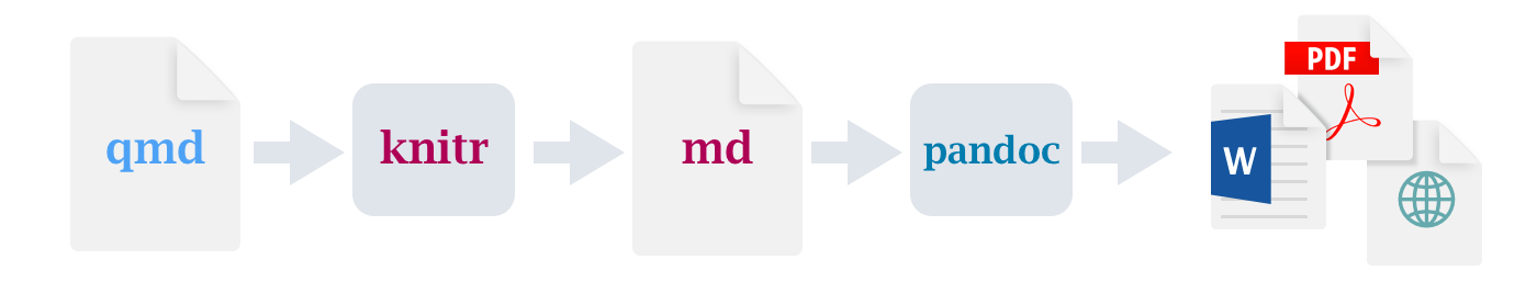
When rendering a document, knitr will execute the R code
in each chunk and creates a new markdown (.md) document,
which will include both the regular text and output from the executed
code chunks. This markdown file is then converted to the final output
format with pandoc. This whole process
is handled for you by the Render button in the RStudio IDE.
Creating a Quarto document
Within RStudio, click
File → New File → Quarto document... and you’ll get a
dialog box like this:
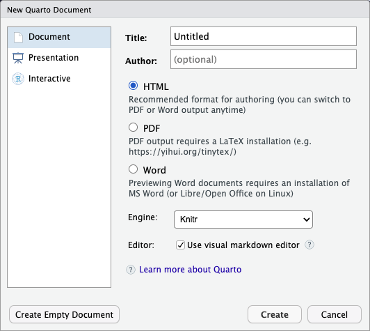
You can stick with the default (HTML output), but give it a title.
Basic components of R Markdown
The initial chunk of text (header) contains instructions for Quarto
to specify what kind of document will be created, and the options
chosen. You can use the header to give your document a title, author,
date, and tell it what type of output you want to produce. In this case,
we’re creating an html document.
You can delete any of those fields if you don’t want them included. The double-quotes aren’t strictly necessary in this case. They’re mostly needed if you want to include a colon in the title.
RStudio creates the document with some example text to get you started. Note below that there are chunks like
```{r}
1 + 1
```
These are chunks of R code that will be executed by
knitr and replaced by their results. More on this
later.
Markdown
Markdown is a system for writing web pages by marking up the text much as you would in an email rather than writing html code. The marked-up text gets converted to html, replacing the marks with the proper html code.
For now, let’s delete all of the stuff that’s there and write a bit of markdown.
You make things bold using two asterisks, like this:
**bold**, and you make things italics by using
underscores, like this: _italics_.
You can make a bulleted list by writing a list with hyphens or asterisks with a space between the list and other text, like this:
MARKDOWN
A list:

* bold with double-asterisks
* italics with underscores
* code-type font with backticks
or like this:
MARKDOWN
A second list:

- bold with double-asterisks
- italics with underscores
- code-type font with backticks
Each will appear as:
- bold with double-asterisks
- italics with underscores
- code-type font with backticks
You can use whatever method you prefer, but be consistent. This maintains the readability of your code.
You can make a numbered list by just using numbers. You can even use the same number over and over if you want:
This will appear as:
- bold with double-asterisks
- italics with underscores
- code-type font with backticks
You can make section headers of different sizes by initiating a line
with some number of # symbols:
You compile the R Markdown document to an html webpage by clicking the “Render” button in the upper-left. Or using the keyboard shortcut Shift+Ctrl+K on Windows and Linux, or Shift+Cmd+K on Mac.
Challenge 1
Create a new Quarto document called “Data analysis with the AMR Package”
Delete all of the R code chunks and write a bit of Markdown (some sections, some italicized text, and an itemized list).
Convert the document to a webpage.
In RStudio, select
File > New file > Quarto Document...
Delete the placeholder text and add the following:
MARKDOWN
# Introduction

## Background on R package

This report uses the **AMR R package** to carry out standardised and reproducible Antimicrobial Resistance (AMR) data analysis.

## Background on the AMR example data set

The AMR package contains a data set called **example_isolates_unclean** which is representative of data extracted directly from microbiology testing laboratories.
Then click the ‘Render’ button on the toolbar to generate an html document (webpage).
A bit more Markdown
You can make a hyperlink like this:
[The AMR Package for R](https://amr-for-r.org/)You can include an image file like this:
You can do subscripts (e.g., F2) with F~2~
and superscripts (e.g., F2) with F^2^.
If you know how to write equations in LaTeX, you can use
$ $ and $$ $$ to insert math equations, like
$E = mc^2$ and
$$y = \mu + \sum_{i=1}^p \beta_i x_i + \epsilon$$which will show as
\[y = \mu + \sum_{i=1}^p \beta_i x_i + \epsilon\]
You can review Markdown syntax by navigating to the “Markdown Quick Reference” under the “Help” field in the toolbar at the top of RStudio.
R code chunks
The real power of Quarto comes from mixing markdown with chunks of code. When processed, the R code will be executed; if they produce figures, the figures will be inserted in the final document.
The main code chunks look like this:
# Loading the required R packages:
```{r}
#| warning: false
library(dplyr)
library(ggplot2)
library(AMR) # load the AMR package

# (if not yet installed, install with:)
# install.packages(c("dplyr", "ggplot2", "AMR"))
```
That is, you place a chunk of R code between ```{r} and
```. You should give each chunk a unique name, by inserting
the line #| label: label_name as they will help you to fix
errors and, if any graphs are produced, the file names are based on the
name of the code chunk that produced them. You can create code chunks
quickly in RStudio using the shortcuts
Ctrl+Alt+I on Windows and Linux, or
Cmd+Option+I on Mac.
In R Markdown, you add chunk labels by including them within the
```{r} line like so:
The AMR package contains a data set called example_isolates_unclean, which is representative of data extracted directly from microbiology testing laboratories:
# Let's have a look at the example_isolates_unclean data set:
```{r}
head(example_isolates_unclean)
```
Challenge 2
In this report we will take this uncleaned data set and prepare it ready for analysis, we would like the microorganism column to contain valid, up-to-date taxonomy, and the antibiotic columns to be cleaned to contain SIR values = Susceptible (standard dose effective), Intermediate (or Susceptible, Increased exposure; requires higher doses), or Resistant (not effective even at higher doses).
Add code chunks to:
- Use chunk for the preparation of uncleaned antimicrobial data sets
- Use the AMR
as.mo()function in AMR to transform arbitrary microorganism names or codes to current taxonomy codes - Use this function to clean up the bacteria column in our data set:
The as.mo() function in AMR can transform arbitrary
microorganism names or codes to current taxonomy codes, this function
supports different types of input for example:
## Taxonomy of microorganisms
```{r}
as.mo("Klebsiella pneumoniae")
```
```{r}
as.mo("K. pneumoniae")
``````{r}
as.mo("KLEPNE")
``````{r}
as.mo("KLPN")
```The first character in output codes denote their taxonomic kingdom, such as Bacteria (B), Fungi (F), and Protozoa (P).
The AMR package also contain functions to directly retrieve taxonomic properties, such as the name, genus, species, family, order, and even Gram-stain:
```{r}
mo_family("K. pneumoniae")
```
```{r}
mo_genus("K. pneumoniae")
``````{r}
mo_species("K. pneumoniae")
``````{r}
mo_gramstain("Klebsiella pneumoniae")
``````{r}
mo_snomed("K. pneumoniae")
```This function can be used to clean up the bacteria column in our data set:
```{r}
AMR_data_unclean <- example_isolates_unclean
AMR_data_unclean$bacteria <- as.mo(AMR_data_unclean$bacteria, info = TRUE)

#ℹ Microorganism translation was uncertain for "E. coli" (assumed Escherichia coli), "S. aureus" (assumed Staphylococcus aureus), and "S. pneumoniae" (assumed Streptococcus pneumoniae). Run mo_uncertainties() to review these uncertainties, or use add_custom_microorganisms() to add custom entries.
We can run this code to check on the taxonomic code translations:
```{r}
mo_uncertainties()
```
How things get compiled
When you press the “Render” button, the Quarto document is processed
by knitr and a plain
Markdown document is produced (as well as, potentially, a set of figure
files): the R code is executed and replaced by both the input and the
output; if figures are produced, links to those figures are
included.
The Markdown and figure documents are then processed by the tool pandoc, which converts the
Markdown file into an html file, with the figures embedded.
Chunk options
There are a variety of options to affect how the code chunks are treated. Here are some examples:
- Use
echo=FALSEto avoid having the code itself shown. - Use
results="hide"to avoid having any results printed. - Use
eval=FALSEto have the code shown but not evaluated. - Use
warning=FALSEandmessage=FALSEto hide any warnings or messages produced. - Use
fig.heightandfig.widthto control the size of the figures produced (in inches).
So you might write:
```{r}
#| label: load_libraries
#| echo: false
#| warning: false
library(dplyr)
library(ggplot2)
library(AMR)
```
Often there will be particular options that you’ll want to use repeatedly; for this, you can set global chunk options in the files YAML header like so:
YAML
---
...
knitr:
  opts_chunk:
    message: false
    warning: false
    echo: false
    results: "hide"
    fig.path: "Figs/"
    fig.width: 11
---
The figures block option defines the path where the
figures will be saved. The / after Figs here is really
important; without it, the figures would be saved in the standard place
but just with names that begin with Figs.
If you have multiple R Markdown files in a common directory, you
might want to use fig.path to define separate prefixes for
the figure file names, like fig.path="Figs/cleaning-" and
fig.path="Figs/analysis-".
You can review all of the R chunk options by navigating
to the “R Markdown Cheat Sheet” under the “Cheatsheets” section of the
“Help” field in the toolbar at the top of RStudio.
Cleaning antibiotic lab test results
The AMR package comes with three new data types to work with such
test results: mic for minimal inhibitory concentrations
(MIC), disk for disk diffusion diameters, and
sir for SIR data that have been interpreted already. This
package can also determine SIR values based on MIC or disk diffusion
values.
This data set just contains SIR data and we want to clean the SIR columns in our data using dplyr:
# Cleaning antibiotic lab test results
```{r}
AMR_data_clean <- AMR_data_unclean %>%
  mutate_if(is_sir_eligible, as.sir)

# mutate_if applies a function to all columns that meet a condition
# is_sir_eligible function returns TRUE if a column contains data that can be interpreted as antimicrobial susceptibility test results (e.g., MIC values, disk diffusion diameters, or categorical "S", "I", "R" results
# as.sir function then takes those eligible columns and converts their values into the "sir" class (standardized "S", "I", "R" format).

AMR_data_clean
```Data inclusion - first isolates
- For analysis of antimicrobial resistance, only the first isolate of every patient per episode should be included (Hindler et al., Clin Infect Dis. 2007).
- If this wasn’t done we would get an overestimate or underestimate of the resistance of an antibiotic.
- For example, if a patient was admitted with an MRSA infection and it was found in five different blood cultures the following weeks . The resistance percentage of oxacillin of all isolates would be overestimated, because you included this MRSA more than once. It would clearly be selection bias.
- The
AMRpackage includes this methodology with thefirst_isolate()function and is able to apply the four different methods as defined by Hindler et al. in 2007: phenotype-based, episode-based, patient-based, isolate-based.
# Data inclusion - first isolates
```{r}
AMR_data_clean <- AMR_data_clean %>%
  mutate(first = first_isolate(info = TRUE))
```
This shows that only 91% of the isoaltes witin this data set are
suitable for resistance analysis! We can now filter using the function
filter_first_isolate()
```{r}
AMR_data_clean_1st <- AMR_data_clean %>%
  filter_first_isolate()

AMR_data_clean_1st
```
We now end up with a cleaned filtered data set with 2,724 isolates for analysis
Data anlysis with the AMR package
- Use the base R
summary()function to get an overview of the cleaned and filtered data set and functionsapplyto get the number of unique values per column. - Report how the species are distributed in the dataset using the
count()funtion. - Select and filter with antibiotic selectors.
Use of the summary() and sapply
functions:
```{r}
summary(AMR_data_clean_1st)

sapply(AMR_data_clean_1st, n_distinct)
```
Use of the count() function
```{r}
AMR_data_clean_1st %>%
  count(mo_name(bacteria), sort = TRUE)
```
We can select/filter columns based on the antibiotic class:
```{r}
AMR_data_clean_1st %>%
  select(date, aminoglycosides())
```
```{r}
AMR_data_clean_1st %>%
select(bacteria, betalactams())
```Resistance percentages
The functions resistance() and susceptibility() can be used to calculate antimicrobial resistance or susceptibility. For more specific analyses, the functions proportion_S(), proportion_SI(), proportion_I(), proportion_IR() and proportion_R() can be used to determine the proportion of a specific antimicrobial outcome.
As per the EUCAST guideline of 2019, we calculate resistance as the proportion of R (proportion_R(), equal to resistance()) and susceptibility as the proportion of S and I (proportion_SI(), equal to susceptibility()).These functions can be used on their own:
```{r}
AMR_data_clean_1st %>% resistance(AMX)
```
Challenge 6
- Use
group_by()andsummarise()from dplyr together with the AMRresistance()function to determine the proportion of isolates that are resistant to amoxicillin for each hospital. - Use the
select()andsummarise()functions together with the AMRresistance()function to determine the resistance proportions by antibiotic. - Use
group_by()andsummarise()functions together with the AMRresistance()function to detmine the resistance proportions by antibiotic and grouped by bacteria.
The proportion of isolates that are resistant to amoxicillin for each hospital:
```{r}
AMR_data_clean_1st %>%
  group_by(hospital) %>%
  summarise(amoxicillin = resistance(AMX))
```
The resistance proportions by antibiotic:
```{r}
AMR_data_clean_1st %>%
  select(AMX, AMC, CIP, GEN) %>%
  summarise(across(everything(), resistance))

```
The resistance proportions by antibiotic and grouped by bacteria:
```{r}
AMR_data_clean_1st %>%
  group_by(bacteria) %>%
  summarise(across(c(AMX, AMC, CIP, GEN), resistance))

```
Inline R code
You can make every number in your report reproducible. Use
`r and ` for an in-line code chunk.
For example we can add in the following for our report:
Using the AMR package example dataset, we analysed `r nrow(AMR_data_clean_1st)` isolates from `r length(unique(AMR_data_clean_1st$bacteria))` different bacterial species.

The overall resistance to ciprofloxacin was `r round(resistance(AMR_data_clean_1st$CIP) * 100, 1)`%.

The most common species was `r AMR_data_clean_1st %>% count(bacteria, sort = TRUE) %>% slice(1) %>% pull(bacteria)`.
Inline example explained:
r nrow(AMR_data_clean_1st) = total number of isolates
r length(unique(AMR_data_clean_1st$bacteria)) = number of species
r round(resistance(AMR_data_clean_1st$CIP) * 100, 1) = calculates the resistance % to CIP
r … %>% count(bacteria, sort = TRUE) = outputs the most frequent species
The code will be executed and replaced with the value of the result.
Don’t let these in-line chunks get split across lines.
Other output options
You can also convert R Markdown to a PDF or a Word document. Change
the format: field in the YAML header to pdf or
docx. For an overview of all the available output formats,
see the Quarto
documentation
Parameterised reports
Literate programming with tools like Quarto and R Markdown is very powerful in that it allows you to generate analysis reports in a reproducible manner. This makes it very easy to update your work and alter the input parameters within the report You can take this one step further, by parametrising the reports themselves. This is very useful in a number of cases, for example:
- Running the same analysis on different datasets
- Generating multiple reports for different groups of the data (e.g. geographic location or time periods)
- Controlling the
knitroptions; e.g. you might want to show the code in some reports but not in others
Including parameters in a Quarto document
Including parameters in a Quarto document (or R Markdown, which
follows the same syntax) can be done by adding the params
field to they YAML header. This field can hold a list of multiple
parameters.
For example, imagine we want to analyse the resistance distribution
using the our AMR_data_clean_1st dataset, but we want a
separate report for each antibiotic. To achieve this, we set the YAML
header for our Quarto document, so if we wanted to calculate the
resistance distribution for Ciprofloxacin, we would do as follows:
YAML
---
---
title: "Data analysis with AMR package"
format: html
editor: visual
params:
  antibiotic: "CIP"
---
We can then reference this parameter anywhere in the R code in our
report by accessing the params object. To visualise the
S/I/R distribution for just the antibiotic defined by the
params, we can do:
```{r}
AMR_data_clean_1st %>%
  ggplot(aes_string(x = params$antibiotic, fill = params$antibiotic)) +
  geom_bar() +
  scale_fill_sir() +
  labs(title = paste(params$antibiotic, "S/I/R distribution"), x = "Interpretation", y = "Count")

```
This code also uses params to set the plot title
Challenge 7
Plot the S/I/R distribution of Ciprofloxacin by hospital using
params
```{r}
AMR_data_clean_1st %>%
  ggplot(aes_string(x = "hospital", fill = params$antibiotic)) +
  geom_bar(position = "fill") +
  scale_fill_sir() +
  labs(title = paste(params$antibiotic, "S/I/R distribution by hospital"),
    x = "Hospital",
    y = "Proportion"
  )

```
Rendering Quarto documents from within R
Of course, manually editing the YAML header every time you want to
generate a report isn’t much better than manually editing the report
itself. The real power of parameterised reports is when we render them
programmatically. This can be done using the {quarto} R
package, which provides the quarto_render() function.
This function takes a Quarto file and any execution parameters as
input.
So to generate the resistance distributions report for Gentamicin, we can write a script with the following code:
R
# render-report.R
library(quarto)
quarto_render("AMR_data_analysis.qmd", execute_params = list(antibiotic = "GEN"))
And now for the real magic, we can modify our script to render a report for a list of antibiotics from the AMR dataset:
# render-all-reports.R
library(quarto)

antibiotics <- c("AMC", "CIP", "GEN", "AMX")

for (ab in antibiotics) {
  quarto_render(
    input = "AMR_data_analysis.qmd",
    output_file = paste0("AMR_", ab, ".html"),
    execute_params = list(antibiotic = ab)
  )
}
After running this script, we should have the following files in our working directory:
.
├── AMR_AMX.html
├── AMR_GEN.html
├── AMR_CIP.html
├── AMR_AMC.html
├── AMR_data_analysis.qmd
WARNING: although this will work and generate the correct output files, you might notice that each report will show the exact same plot, which is unexpected. This is an issue with the Quarto R package.
With R Markdown we don’t have this issue, to render we would use the following code:
R
library(rmarkdown)

antibiotics <- c("AMC", "CIP", "GEN", "AMX")

for (ab in antibiotics) {
  render(
    input = "AMR_data_analysis.Rmd",
    output_file = paste0("AMR_", ab, ".html"),
    params = list(antibiotic = ab),
    envir = new.env()  # avoids parameter bleed between runs
  )
}
Challenge 8
Use params and the AMR package function
resistance_predict to predict the resistance trends for one
antibiotic
```{r}
params$antibiotic_trend <- resistance_predict(
  x = AMR_data_clean_1st,   # <- your dataset
  col_ab = params$antibiotic, # column with S/I/R
  col_date = "date",        # column with Date
  model = "binomial",       # logistic regression
  year_max = 2025           # optional
)

# plot for one antibiotic

ggplot(params$antibiotic_trend, aes(x = year, y = observed)) +
  geom_point() +
  geom_line(aes(y = estimated), color = "purple") +
  geom_ribbon(aes(ymin = se_min, ymax = se_max), alpha = 0.2, fill = "purple") +
  scale_y_continuous(labels = scales::percent) +
  labs(
    title = paste(params$antibiotic, "Resistance Trend"),
    x = "Year",
    y = "Resistance (%)"
  ) +
  theme_minimal()

```
```r
In an R Script, use to change antibiotic:
# render-report.R
library(quarto)
quarto_render("AMR_data_analysis.qmd", execute_params = list(antibiotic = "GEN"))
```Tip: Creating PDF documents
Creating .pdf documents may require installation of some extra
software. The R package tinytex provides some tools to help
make this process easier for R users. With tinytex
installed, run tinytex::install_tinytex() to install the
required software (you’ll only need to do this once) and then when you
knit to pdf tinytex will automatically detect and install
any additional LaTeX packages that are needed to produce the pdf
document. Visit the tinytex
website for more information.
Tip: Visual markdown editing in RStudio
RStudio versions 1.4 and later include visual markdown editing mode.
In visual editing mode, markdown expressions (like
**bold words**) are transformed to the formatted appearance
(bold words) as you type. This mode also includes a
toolbar at the top with basic formatting buttons, similar to what you
might see in common word processing software programs. You can turn
visual editing on and off by pressing the ![]() button in the top right corner of your R Markdown document.
button in the top right corner of your R Markdown document.
Resources
- Knitr in a knutshell tutorial
- Dynamic Documents with R and knitr (book)
- R Markdown documentation
- R Markdown cheat sheet
- Getting started with R Markdown
- R Markdown: The Definitive Guide (book by Rstudio team)
- Reproducible Reporting
- The Ecosystem of R Markdown
- Introducing Bookdown
Challenge: Quarto presentation
Using what you have learned about Quarto create a new Quarto Presentation.
Present your findings of key factors influencing antimicrobial resistance, this should include:
- text
- plots
Make use of embedded code chunks where appropriate.
- Mix reporting written in R Markdown with software written in R.
- Specify chunk options to control formatting.
- Use
knitrto convert these documents into PDF and other formats.