Week 3 - Running Examples & Preparing Outputs

03 Jul 2026 - Tanvir Islam - learning, python, tutorials, examples

Highlights From This Week

At last, this week I managed to run some of the S2FFT examples from the existing documentation.

Although I still don’t fully understand all the mathematical concepts behind the package, I was able to gain a much deeper intuition by actually running the package and varying different parameters and inputs, and observing how the output was affected.

A good starting point was the round-trip test: generating a random bandlimited signal, mapping it to the sphere with the inverse transform, and then transforming it straight back with the forward transform. Checking that the recovered coefficients matched the originals (to near machine precision) was a simple but reassuring way to confirm I had everything set up correctly and that I understood which direction each transform goes.

From there I started varying things to see what happened:

• Bandlimit (L): I’ve started to understand how varying the bandlimit affects both accuracy and cost — higher L captures finer detail on the sphere but noticeably increases compute time and memory usage.
• Sampling schemes: I compared different sampling schemes, such as the McEwen & Wiaux (MW) scheme and HEALPix. The equiangular MW sampling has an exact sampling theorem, so its round-trip error stays close to machine precision, whereas HEALPix doesn’t, and so it shows a small error. HEALPix trades that exactness for equal-area pixels. It was useful to see that trade-off in practice rather than just reading about it.
• Numerical precision: I also noticed the effect of enabling 64-bit precision in JAX. Leaving it on the default 32-bit made the round-trip error much larger even at moderate L.

Alongside the code, I spent some time skimming the Price & McEwen paper that the package is based on, mainly to get a rough feel for where the recursions come from, even if the details are beyond me for now.

Plan For Next Week

Hopefully next week I can start planning some of the tutorial documentation. In order to do that, I plan to familiarise myself with the visualisation tooling I’ll need to present these transforms clearly:

• matplotlib, as the foundation for plotting.
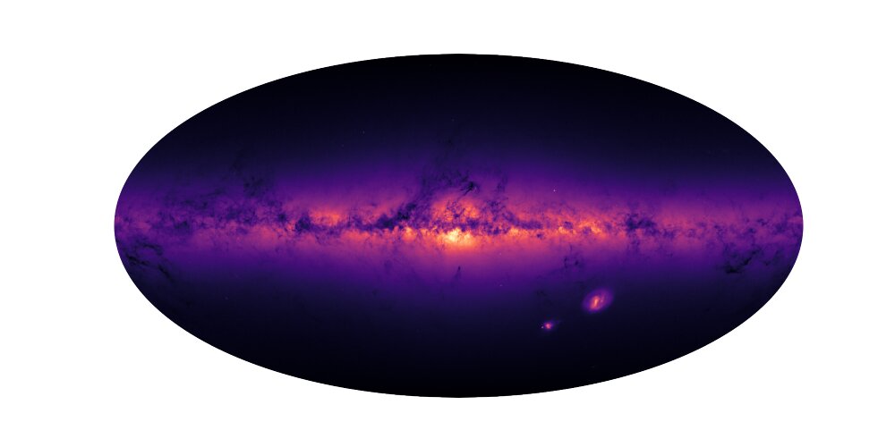
• cartopy, which the existing examples use to show maps on the sphere via projections like Mollweide.
• 3D visualisation libraries such as plotly, PyVista, or Mayavi, so I can show signals wrapped onto an actual sphere rather than a flat projection.
• healpy, for visualising signals in the HEALPix sampling scheme specifically.

Once I’m comfortable with those, I’d like to sketch out a rough structure for a tutorial.