Assumption Diagnostics and Regression Trouble Shooting

Last updated on 2024-09-04 | Edit this page

Overview

Questions

How can I check that my data is suitable for use in a linear regression model?

Objectives

To be able to check assumptions for linear regression models

Content

Residual diagnostics
Heteroskedasticity Check
Multicollinearity Check
Identification of Influential Points

Data

R

# We will need these libraries and this data later.
library(ggplot2)
library(olsrr)
library(car)

lon_dims_imd_2019 <- read.csv("data/English_IMD_2019_Domains_rebased_London_by_CDRC.csv")

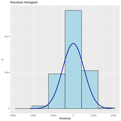
For accurate model interpretation and prediction, there are a number of assumptions about linear regression models that need to be verified. These are: * Linear Relationship: The core premise of multiple linear regression is the existence of a linear relationship between the dependent (outcome) variable and the independent variables. T * Multivariate Normality: The analysis assumes that the residuals (the differences between observed and predicted values) are normally distributed. This assumption can be assessed by examining histograms or Q-Q plots of the residuals, or through statistical tests such as the Kolmogorov-Smirnov test. * No Multicollinearity: It is essential that the independent variables are not too highly correlated with each other, a condition known as multicollinearity. This can be checked using: + Correlation matrices, where correlation coefficients should ideally be below 0.80. + Variance Inflation Factor (VIF), with VIF values above 10 indicating problematic multicollinearity. * Homoscedasticity: The variance of error terms (residuals) should be consistent across all levels of the independent variables.

We can perform a number of tests to see if the assumptions are met.

Residual Diagnostics

Residual QQ Plot

Plot for detecting violation of normality assumption.

R

model1 <- lm(health_london_rank ~ livingEnv_london_rank + barriers_london_rank + la19nm, data = lon_dims_imd_2019)

ols_plot_resid_qq(model1)

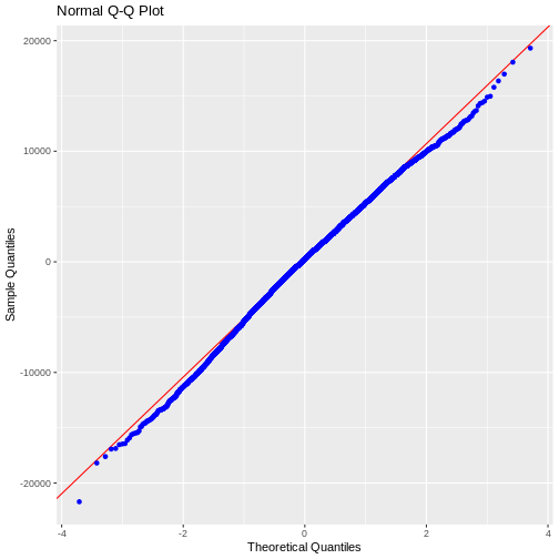
Residual Normality Test

Test for detecting violation of normality assumption.

R

ols_test_normality(model1)

OUTPUT

-----------------------------------------------
       Test             Statistic       pvalue
-----------------------------------------------
Shapiro-Wilk              0.9968         0.0000
Kolmogorov-Smirnov        0.0238         0.0084
Cramer-von Mises         404.803         0.0000
Anderson-Darling          4.1283         0.0000
-----------------------------------------------

Correlation between observed residuals and expected residuals under normality.

R

ols_test_correlation(model1)

OUTPUT

[1] 0.9983931

From these tests we can see that our assumptions are seemingly correct.

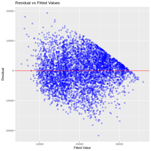
Residual vs Fitted Values Plot

We can create a scatter plot of residuals on the y axis and fitted values on the x axis to detect non-linearity, unequal error variances, and outliers.

Characteristics of a well behaved residual vs fitted plot: * The residuals spread randomly around the 0 line indicating that the relationship is linear. * The residuals form an approximate horizontal band around the 0 line indicating homogeneity of error variance. * No one residual is visibly away from the random pattern of the residuals indicating that there are no outliers.

R

ols_plot_resid_fit(model1)

Residual Histogram

Additionally, we can create a histogram of residuals for detecting violation of normality assumption.

R

ols_plot_resid_hist(model1)

Additional Diagnostics

In addition the residual diagnostics, we can also assess our model for Heteroskedasticity, Multicollinearity and any Influential/High leverage points.

Heteroskedasticity Check

We can use the ncvTest() function to test for equal variances.

R

ncvTest(model1)

OUTPUT

Non-constant Variance Score Test
Variance formula: ~ fitted.values
Chisquare = 52.92299, Df = 1, p = 3.4689e-13

The p-value here is low, indicating that this model may have a problem of unequal variances.

Multicollinearity Check

We want to know whether we have too many variables that have high correlation with each other. If the value of GVIF is greater than 4, it suggests collinearity.

R

vif(model1)

OUTPUT

                          GVIF Df GVIF^(1/(2*Df))
livingEnv_london_rank 1.790038  1        1.337923
barriers_london_rank  2.038530  1        1.427771
la19nm                3.583479 32        1.020143

Outlier Identification

We can identify outliers in our data by creating a QQPlot and running statistical tests on the data. The outlierTest() reports the Bonferroni p-values for testing each observation in turn to be a mean-shift outlier, based Studentized residuals in linear (t-tests), generalized linear models (normal tests), and linear mixed models.

R

# Create a qqPlot
qqPlot(model1, id.n = 2)

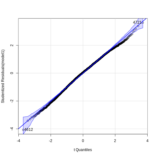
OUTPUT

[1] 4612 4721

R

# Test for outliers
outlierTest(model1)

OUTPUT

No Studentized residuals with Bonferroni p < 0.05
Largest |rstudent|:
      rstudent unadjusted p-value Bonferroni p
4612 -4.069694         4.7832e-05      0.23127

The null hypothesis for the Bonferonni adjusted outlier test is the observation is an outlier. Here observation related to ‘4612’ is an outlier. In our data ‘4612’ is difficult to identify as it may refer to either a Living Environment or a Barriers rank.

Identifying Influence Points

We can identify potential influential points via an Influence Plot, these may be Ouliers and/or High Leverage points. A point can be considered influential if it’s exclusion causes substantial change in the estimated regression.

An influence plot summarises the 3 metrics for influence analysis in one single glance. The X-axis plots the leverage, which is normalised between 0 and 1. The Y-axis plots the studentized residuals, which can be positive or negative. The size of the circles for each data point reflect its Cook’s distance, degree of influence.

Vertical reference lines are drawn at twice and three times the average hat value, horizontal reference lines at -2, 0, and 2 on the Studentized-residual scale.

R

# Influence Plots
influencePlot(model1)

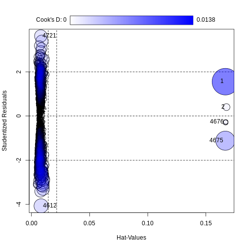
OUTPUT

        StudRes         Hat        CookD
1     1.5548629 0.166808357 0.0138248622
2     0.4024213 0.167706627 0.0009324887
4612 -4.0696939 0.008281120 0.0039386753
4675 -1.1177591 0.166718323 0.0071416294
4676 -0.2645859 0.167101314 0.0004013628
4721  3.6227234 0.007981167 0.0030092149

Identified influential points are returned in a data frame with the hat values, Studentized residuals and Cook’s distance of the identified points. If no points are identified, nothing is returned.

Influence points can be further explored with an Influence Index Plot which provides index plots of influence and related diagnostics for a regression model.

R

influenceIndexPlot(model1)

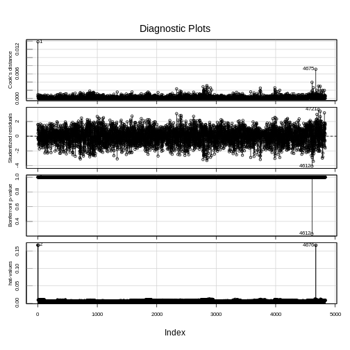
If an observation is influential then that observation can change the fit of the linear model.

An observation may be influential because: 1. Someone made a recording error 2. Someone made a fundamental mistake collecting the observation 3. The data point is perfectly valid, in which case the model cannot account for the behaviour.

If the case is 1 or 2, then you can remove the point (or correct it). If it’s 3, it’s not worth deleting a valid point; the data may be better suited a non-linear model.

Challenge

Choose 3 of the of the regression diagnostics, check that the assumptions are met for the linear models you have created using the gapminder data.

State what you tested and discuss your findings.